How a Python SQL Engine Got to the Top of ClickBench

TL;DR

• Opteryx plans queries in Python. The work on the data is done in native code: Cython, C++ and a little Rust.
• On ClickBench, with the storage filter set to Parquet, Opteryx 0.9.167 is first of 41 entries on c6a.large, for both the hot and the combined score (14 October 2026). On bigger machines it's third, and further down on cold runs.
• We didn't get there with one trick. We got there by measuring everything, re-running the same tests on different CPUs, trying ideas just to see what happens, and working on every layer of the engine.

Python plans, native code runs

Opteryx is a Python package. You pip install opteryx-core, import opteryx, and give it SQL. Parsing, binding and optimizing the query all run in Python.

After that, Python steps aside. The planner hands the physical plan to the native executor once, and the executor never calls back into Python to make a decision. Readers, vectors, expressions, joins and aggregations are all native code. Operators run on worker threads with the interpreter lock released. A query that touches 100 million rows spends almost no time in Python, because there's very little Python left on that path.

We split it this way on purpose. Planning is where the engine makes decisions: which join order to use, which estimate to trust, whether a filter can move below a join. It's branchy, full of special cases, and the least deterministic part of the engine. It's also where a lot of our speed experiments happen: a new rewrite rule or a better estimate changes how much work execution has to do. Python is faster to reason about. When the planner makes an odd choice, it's quick to work out why, and quick to try something different.

Moving data is the opposite: the same few operations, billions of times, where every byte and branch counts. C++ is good at being fast, so that's where it goes.

It turns out the planning cost is small. On ClickBench's hot runs, on both c6a.large and c6a.4xlarge, several of the simplest queries finish in 3 to 4 milliseconds, Python planning included.

Where Opteryx ranks

ClickBench is a lot of benchmarks in one. There are nine machine types, three scores (cold, hot and combined), and filters for how the data is stored. The result depends on which of those you pick. This is the view where Opteryx comes first:

Machine	c6a.large (2 vCPU, 4 GB RAM)
Storage filter	Parquet
Entry	Opteryx, opteryx-core 0.9.167, 14 October 2026
Position	1st of 41 on combined, 1st of 43 on hot

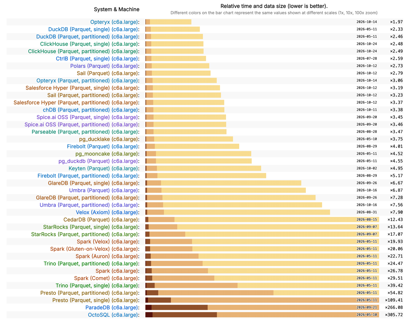
ClickBench, c6a.large, storage filter Parquet, combined score, captured 24 October 2026. Lower is better. The leaderboard changes as entries are re-run; the live view shows where things stand today.

Some context for that result:

• That entry rewrites the data first. The load step rewrites ClickBench's Parquet files using Opteryx's own Parquet writer, sorted by the primary key the rules allow, and that time counts as load time. Our other entry reads the files as shipped, and on the same view it comes ninth.
• The score is a geometric mean of per-query ratios. That rewards being quick on most queries more than it punishes being terrible on a few, and we benefit from that here. On 4 GB of RAM, four of the heaviest GROUP BY queries spill to swap, and their hot runs take between 16 and 51 minutes. DuckDB, reading the same Parquet, finishes each of them in 21 to 31 seconds.
• Results are snapshots. Entries get re-run at different times. The two DuckDB entries just behind us on that machine were last run in May.
• Bigger machines are harder. On c6a.4xlarge, c6a.2xlarge and c8g.4xlarge we're third, behind both Pivotlake entries. On the Graviton metal machine we're fifth, and on the two AMD metal machines eighth to tenth. On cold runs we're mid-pack everywhere.

On a small machine, an engine with a Python front end is faster than every other Parquet engine on most of the queries. That surprised us as much as anyone. The rest of this post is about how it happened.

We measure everything, all the time

You can't improve something you aren't watching. Opteryx runs nine performance suites against itself: TPC-H, TPC-DS, ClickBench, JOB, H2O, JSONBench, and three of our own built from queries we've seen users run. Benchmark queries and real queries aren't the same shape, and it's the real ones we have to be fast at. We also run four correctness suites. The benchmarking page has the full list. Here's why we run so many and how we run them.

Many suites, so we don't overfit to one. If ClickBench were the only benchmark we ran, we'd have a fast scanner and a bad optimizer. ClickBench barely tests join ordering. JOB tests almost nothing else. Each suite exists because another one couldn't see a particular kind of failure. We wrote about what each one found the first time we ran it.

Every run is kept. Each iteration is written to results/<git-sha>-<timestamp>.csv. When a query gets slower, we can bisect it to the commit that did it, without trying to remember what the numbers used to be.

Same conditions every time. Each query runs several times in a fresh session and we compare the best time. The result is drained without rendering, so we measure the engine, not the table formatter. Benchmarks preload the same memory allocator as the production build, so local numbers and deployed numbers mean the same thing.

A fixed reference. Most suites compare against a DuckDB baseline that is measured on the same machine and only refreshed on purpose. A baseline that moves on every run makes every comparison meaningless.

Release over release. Wrenchy Bench re-runs the suites on AWS Graviton4 for each release. The ClickBench run went from 29.44 s at its slowest to 15.41 s as of 0.9.155, over 48 recorded runs. That trend tells us more than any single ranking does.

Telemetry inside the planner. Measuring speed isn't enough. We also record which path the engine took. When the optimizer uses a new estimator, telemetry records whether it fired or fell back to the default. So the fallback rate is a number we can see, not one we assume.

We A/B test across architectures

Opteryx is developed on Apple Silicon laptops (ARM), runs in production on x86, is tracked release over release on Graviton4 (ARM again), and gets benchmarked on ClickBench's AMD and Graviton fleet. We've also run it on a RISC-V board for fun.

These machines regularly disagree. A change that helps on an M-series laptop, with its huge caches and memory bandwidth, can do nothing or even hurt on a 2-vCPU x86 cloud instance. So a change isn't finished when it's faster on the machine it was written on. It's finished when it's faster on the machines people actually use.

When we compare two versions, we compare them properly. When we were choosing a row-group size, we rewrote TPC-H at five sizes and ran all 22 queries with the versions interleaved. We also rotated their order each round, so a warming cache or a noisy neighbour couldn't favour whichever version ran last.

The ClickBench results show why this matters. The same build is first on a 2-core AMD machine, third on a 16-core Graviton, and ninth on a 192-core one. If we only looked at one machine, we'd learn one of those facts and miss the other two. The last one is the most useful to us: it says we have work to do on scaling across many cores.

We try things just to see if they work

A lot of what got us here began as "I wonder if…". Most of those experiments fail. That's fine. A failed experiment that takes an afternoon is cheap, and the ones that work are often things nobody would have planned for.

Some of them:

• A RISC-V board. We did it for no particularly good reason, and with no plan. It found SIMD code that had never been compiled, a signed-versus-unsigned bug in a hex decoder, and missing #includes that Apple's toolchain had been quietly covering for. Every one of those fixes made the x86 and ARM builds better too.
• Our own hash table versus Abseil. Ours won on build time and lost on probe time. Changing the layout and adding prefetching took about 30% off probe latency. A partial win, and we learned exactly where the cost was.
• Several ways to guess LIKE selectivity. Entropy, Markov bigrams (at full precision, fp16 and 8-bit), averages of models, clamping. Most of them lost to a plain character-class model. The bigram model was the most sophisticated, and it lost because its noise correction smoothed away real signal.
• A file format of our own. Skene is still a draft and not something we recommend for production. On Wrenchy Bench it runs ClickBench in 10.89 s, against 15.41 s for Parquet on the same machine. That gap shows how much file layout matters, and it gives the Parquet path a target.

The rule is simple: an idea gets tested by running it, not by arguing about it. If it doesn't work, we write down why and move on.

We work at every layer

There was no single big speedup. There were many small ones at every level, from how bytes sit in a file to how the optimizer guesses row counts. Here are the main layers, from the bottom up.

File layout

The fastest byte is the one you never read. Owning the Parquet writer means we decide what's in the file. That includes dictionary encoding where it pays off, bloom filters, and sorted dictionary keys, so some range filters become integer comparisons on dictionary codes. On the reading side, projection, row-group pruning and dictionary skipping all happen before any value is decoded.

We also split one setting into two. Row-group size used to set both how many requests we make to object storage and how big each unit of engine work is. Those want different values. Now we write 64k-row row groups in blocks of four. The engine gets smaller units of work, and object storage still gets large reads.

This is also why the ClickBench entry with the load step ranks higher than the one that reads the shipped files. The data is the same. The layout is better.

Memory allocation

Allocations are expensive and they hide well. Some of the larger wins we've had came from not allocating at all:

• Aggregates used to turn column values into Python objects so they could be summed. Doing it natively over the raw buffers made them 10–100× faster.
• The memory pool kept its bookkeeping in Python dictionaries. Moving that into a compact C++ structure gave 10× the throughput, without changing its API.
• The JSON reader used to make one allocation per record. Now it builds one contiguous arena for the whole batch. That's what made SELECT * over JSON competitive.
• The expression engine works out the maximum stack depth while it compiles an expression, and allocates that space once. Temporary results come from a per-batch arena that is freed all at once.

Cache lines

Once allocations are gone, the next limit is usually how far data has to travel to reach the CPU.

• Strings are stored in 16-byte slots. Strings of 12 bytes or fewer live entirely inside the slot. Longer ones keep their length and first four bytes there. Most equality checks are settled by one 64-bit compare, and ordering by a 4-byte prefix, without fetching a second cache line.
• Small integer sets use a direct-addressed bit array instead of a hash table. Its size is capped at 262,144 slots, which is 32 KB and fits in L1 cache. Above that size, it stops being faster than the hash table it replaces.
• Hash table probes were limited by L1 and L2 cache misses, not by computation. Changing the layout and prefetching likely buckets ahead of time helped more than any change to the hash function.
• Morsel size, the number of rows each worker handles at once, decides whether that batch fits in cache. That's why we measured it rather than inheriting the number from storage.

Expressions

The old expression evaluator walked a tree of Python objects and re-made the same decisions for every batch. Its bytecode replacement makes those decisions once, when the query is planned. It binds each operation to a native function, turns literals into constant vectors, and runs a flat list of instructions. The executor's job is just to run what's already been decided.

The optimizer's estimates

An optimizer is only as good as its guesses about row counts. A plan built on a bad estimate still returns the right answer, just slowly. JOB is the suite that shows this most clearly. The engine can be fast at every step and still pick a join order that does many times more work than it needed to.

So we treat estimates as something to measure. Every LIKE '%needle%' used to be assumed to match 10% of rows. We tested several replacement estimators against real data and shipped one that cut the mean absolute error from 14.5% to 4.45%. Along the way we found the statistics pipeline was writing empty columns where min, max, null counts and histograms should have been. We fixed that too, with native code.

This is the least glamorous layer and probably the one with the most room left. Every wrong estimate costs time on every query that depends on it.

What's left

Plenty. Cold runs are bound by storage, and we're mid-pack on them. Heavy GROUP BY queries that don't fit in memory spill badly. On c6a.large's hot runs, those four queries take about 6,300 seconds between them, and the other 39 take 86. On c6a.4xlarge, with 32 GB, they don't spill: the same four take 7.5 seconds, against 12.9 for the rest, and they're about level with DuckDB. The work is in making the spill path degrade gracefully instead of falling off a cliff. And the drop from first on 2 cores to ninth on 192 cores tells us where to look next.

All of those came from the same habits that got us this far. We'll keep measuring, keep testing on more than one machine, and keep trying things.

Engineering takeaways

• Python in the planner is fine. Keep it off the data path and its cost hardly shows.
• Run many benchmarks. Any single benchmark rewards overfitting to it.
• Keep every result. If you can't bisect a regression, you're relying on memory.
• Test on the machines your users run. Your laptop isn't one of them.
• Try things cheaply, and write down the failures.
• Work every layer. The big speedups are usually lots of small ones stacked together.
• Name the machine and the view with every result. Show the slow queries too.

— Justin